A New Link to an Old Model Could Crack the Mystery of Deep Learning

Olena Shmahalo/Quanta Magazine
Introduction
In the machine learning world, the sizes of artificial neural networks — and their outsize successes — are creating conceptual conundrums. When a network named AlexNet won an annual image recognition competition in 2012, it had about 60 million parameters. These parameters, fine-tuned during training, allowed AlexNet to recognize images that it had never seen before. Two years later, a network named VGG wowed the competition with more than 130 million such parameters. Some artificial neural networks, or ANNs, now have billions of parameters.
These massive networks — astoundingly successful at tasks such as classifying images, recognizing speech and translating text from one language to another — have begun to dominate machine learning and artificial intelligence. Yet they remain enigmatic. The reason behind their amazing power remains elusive.
But a number of researchers are showing that idealized versions of these powerful networks are mathematically equivalent to older, simpler machine learning models called kernel machines. If this equivalence can be extended beyond idealized neural networks, it may explain how practical ANNs achieve their astonishing results.
Part of the mystique of artificial neural networks is that they seem to subvert traditional machine learning theory, which leans heavily on ideas from statistics and probability theory. In the usual way of thinking, machine learning models — including neural networks, trained to learn about patterns in sample data in order to make predictions about new data — work best when they have just the right number of parameters.
If the parameters are too few, the learned model can be too simple and fail to capture all the nuances of the data it’s trained on. Too many and the model becomes overly complex, learning the patterns in the training data with such fine granularity that it cannot generalize when asked to classify new data, a phenomenon called overfitting. “It’s a balance between somehow fitting your data too well and not fitting it well at all. You want to be in the middle,” said Mikhail Belkin (opens a new tab), a machine learning researcher at the University of California, San Diego.
By all accounts, deep neural networks like VGG have way too many parameters and should overfit. But they don’t. Instead, such networks generalize astoundingly well to new data — and until recently, no one knew why. It wasn’t for lack of trying. For example, Naftali Tishby, a computer scientist and neuroscientist at the Hebrew University of Jerusalem who died in August, argued that deep neural networks first fit the training data and then discard irrelevant information (by going through an information bottleneck (opens a new tab)), which helps them generalize. But others have argued (opens a new tab) that this doesn’t happen in all types of deep neural networks, and the idea remains controversial.
Now, the mathematical equivalence of kernel machines and idealized neural networks is providing clues to why or how these over-parameterized networks arrive at (or converge to) their solutions. Kernel machines are algorithms that find patterns in data by projecting the data into extremely high dimensions. By studying the mathematically tractable kernel equivalents of idealized neural networks, researchers are learning why deep nets, despite their shocking complexity, converge during training to solutions that generalize well to unseen data.
“A neural network is a little bit like a Rube Goldberg machine. You don’t know which part of it is really important,” said Belkin. “I think reducing [them] to kernel methods — because kernel methods don’t have all this complexity — somehow allows us to isolate the engine of what’s going on.”
Find the Line
Kernel methods, or kernel machines, rely on an area of mathematics with a long history. It goes back to the 19th-century German mathematician Carl Friedrich Gauss, who came up with the eponymous Gaussian kernel, which maps a variable x to a function with the familiar shape of a bell curve. The modern usage of kernels took off in the early 20th century, when the English mathematician James Mercer used them for solving integral equations. By the 1960s, kernels were being used in machine learning to tackle data that was not amenable to simple techniques of classification.
Understanding kernel methods requires starting with algorithms in machine learning called linear classifiers. Let’s say that cats and dogs can be classified using data in only two dimensions, meaning that you need two features (say the size of the snout, which we can plot on the x-axis, and the size of the ears, which goes on the y-axis) to tell the two types of animals apart. Plot this labeled data on the xy-plane, and cats should be in one cluster and dogs in another.
One can then train a linear classifier using the labeled data to find a straight line that separates the two clusters. This involves finding the coefficients of the equation representing the line. Now, given new unlabeled data, it’s easy to classify it as a dog or a cat by seeing which side of the line it falls on.
Dog and cat lovers, however, would be aghast at such oversimplification. Actual data about the snouts and ears of the many types of cats and dogs almost certainly can’t be divided by a linear separator. In such situations, when the data is linearly inseparable, it can be transformed or projected into a higher-dimensional space. (One simple way to do this would be to multiply the value of two features to create a third; maybe there is something about the correlation between the sizes of the snouts and ears that separates dogs from cats.)
More generally, looking at the data in higher-dimensional space makes it easier to find a linear separator, known as a hyperplane when the space has more than three dimensions. When this hyperplane is projected back to the lower dimensions, it’ll take the shape of a nonlinear function with curves and wiggles that separates the original lower-dimensional data into two clusters.
When we’re working with real data, though, it’s often computationally inefficient — and sometimes impossible — to find the coefficients of the hyperplane in high dimensions. But it isn’t for kernel machines.
Kernel of Truth
The power of kernel machines involves their ability to do two things. First, they map each point in a low-dimensional data set to a point that lives in higher dimensions. The dimensionality of this hyperspace can be infinite, depending on the mapping, which can pose a problem: Finding the coefficients of the separating hyperplane involves calculating something called an inner product for each pair of high-dimensional features, and that becomes difficult when the data is projected into infinite dimensions.
Samuel Velasco/Quanta Magazine
So here’s the second thing kernel machines do: Given two low-dimensional data points, they use a kernel function to spit out a number that’s equal to the inner product of the corresponding higher-dimensional features. Crucially, the algorithm can use this trick to find the coefficients of the hyperplane, without ever actually stepping into the high-dimensional space.
“The great thing about the kernel trick is that all the computations happen in the low-dimensional space” rather than the possibly infinite-dimensional space, said Bernhard Boser (opens a new tab), a professor emeritus at the University of California, Berkeley.
Boser, together with his colleagues Isabelle Guyon (opens a new tab) and Vladimir Vapnik (opens a new tab), invented a class of kernel machines called support vector machines (SVMs) (opens a new tab) in the late 1980s and early 1990s, when they were all at Bell Labs in Holmdel, New Jersey. While kernel machines of various types had made their mark in machine learning from the 1960s onward, it was with the invention of SVMs that they took center stage. SVMs proved extraordinarily powerful. By the early 2000s, they were used in fields as diverse as bioinformatics (for finding similarities between different protein sequences and predicting the functions of proteins, for example), machine vision and handwriting recognition.
SVMs went on to dominate machine learning until deep neural networks came of age in 2012 with the arrival of AlexNet. As the machine learning community pivoted to ANNs, SVMs were left stranded, but they (and kernel machines generally) remain powerful models that have much to teach us. For example, they can do more than just use the kernel trick to find a separating hyperplane.
“If you have a powerful kernel, then you are mapping the data to a kernel space that is kind of infinite-dimensional and very powerful,” said Chiyuan Zhang (opens a new tab), a research scientist at Google Research’s Brain Team. “You can always find a linear separator in this powerful hidden space that separates the data, and there are infinitely many possible solutions.” But kernel theory lets you pick not just an arbitrary linear separator, but the best possible one (for some definition of “best”), by limiting the space of solutions to search. This is akin to reducing the number of parameters in a model to prevent it from overfitting, a process called regularization. Zhang wondered if deep neural networks might be doing something similar.
Deep neural networks are made of layers of artificial neurons. They have an input layer, an output layer and at least one hidden layer sandwiched between them. The more hidden layers there are, the deeper the network. The parameters of the network represent the strengths of the connections between these neurons. Training a network for, say, image recognition involves repeatedly showing it previously categorized images and determining values for its parameters that help it correctly characterize those images. Once trained, the ANN represents a model for turning an input (say, an image) into an output (a label or category).
In 2017, Zhang and colleagues carried out a series of empirical tests on networks (opens a new tab) like AlexNet and VGG to see whether the algorithms that are used to train these ANNs are somehow effectively reducing the number of tunable parameters, resulting in a form of implicit regularization. In other words, did the training regime render these networks incapable of overfitting?
The team found that this was not the case. Using cleverly manipulated data sets, Zhang’s team showed that AlexNet and other such ANNs are indeed capable of overfitting and not generalizing. But the same networks trained with the same algorithm didn’t overfit — rather, they generalized well — when given unaltered data. This kind of implicit regularization couldn’t be the answer. The finding called for “a better explanation to characterize generalization in deep neural networks,” said Zhang.
Infinite Neurons
Meanwhile, studies (opens a new tab) were showing that wider neural networks are typically as good or better at (opens a new tab) generalization than their narrower counterparts. To some this was a hint that maybe ANNs could be understood by adopting a strategy from physics, where “studying limiting cases can sometimes simplify a problem,” said Yasaman Bahri (opens a new tab), a research scientist on Google Research’s Brain Team. To tackle such situations, physicists often simplify the problem by considering extreme cases. What happens when the number of particles in a system goes to infinity, for example? “Statistical effects can become easier to deal with in those limits,” said Bahri. What would happen to a neural network, mathematically speaking, if the width of its layers — the number of neurons in a single layer — were infinite?
In 1994, Radford Neal, now a professor emeritus at the University of Toronto, asked this exact question of a network with a single hidden layer. He showed that if the weights of this network were set up, or initialized, with certain statistical properties, then at initialization (before any training), such a network was mathematically equivalent (opens a new tab) to a well-known kernel function called a Gaussian process. More than two decades later, in 2017, two groups, including Bahri’s, showed (opens a new tab) that the same holds true of idealized infinite-width deep neural networks with many hidden layers.
This had a startling implication. Usually, even after a deep net has been trained, an analytical mathematical expression cannot be used to make predictions about unseen data. You just have to run the deep net and see what it says — it’s something of a black box. But in the idealized scenario, at initialization the network is equivalent to a Gaussian process. You can throw away your neural network and just train the kernel machine, for which you have the mathematical expressions.
“Once you map it over to a Gaussian process … you can calculate analytically what the prediction should be,” said Bahri.
This was already a landmark result, but it didn’t mathematically describe what happens during the most common form of training used in practice. In this latter setting, it was unclear how the solution could generalize so well.
Begin the Descent
Part of the mystery centered on how deep neural networks are trained, which involves an algorithm called gradient descent. The word “descent” refers to the fact that, during training, the network traverses a complex, high-dimensional landscape full of hills and valleys, where each location in the landscape represents the error made by the network for a given set of parameter values. Eventually, once the parameters have been suitably tuned, the ANN reaches a region called the global minimum, meaning it’s as close as possible to accurately classifying the training data. Training a network is essentially a problem of optimization, of finding the global minimum, with the trained network representing an almost optimal function that maps inputs to outputs. It’s a complex process that’s difficult to analyze.
“No existing theory can guarantee that if you apply some widely used algorithm like gradient descent, [the ANN] can converge to the global minimum,” said Simon Du (opens a new tab), an expert on machine learning at the University of Washington in Seattle. By the end of 2018, we began to understand why.
Again, as often happens with major scientific advances, multiple groups arrived at a possible answer at the same time, based on mathematical analyses of infinite-width networks and how they relate to the better-understood kernel machines. Around the time Du’s group and others put out papers, a young Swiss graduate student named Arthur Jacot (opens a new tab) presented his group’s work (opens a new tab) at NeurIPS 2018, the field’s flagship conference.
While the teams differed in the details and the framing of their work, the essence was this: Deep neural networks of infinite width, whose weights are initialized with certain statistical properties in mind, are exactly equivalent to kernels not just at initialization, but throughout the training process. A key assumption about the weights is that they individually change very little during training (though the net effect of an infinite number of small changes is significant). Given such assumptions, Jacot and his colleagues at the Swiss Federal Institute of Technology Lausanne showed that an infinite-width deep neural network is always equivalent to a kernel that never changes during training. It does not even depend on the training data. The kernel function depends only on the architecture of the neural network, such as its depth and type of connectivity. The team named their kernel the neural tangent kernel, based on some of its geometric properties.
“We know that at least in some cases neural networks can behave like kernel methods,” said Jacot. “It’s the first step to try to really compare these methods in trying to understand the similarities and differences.”
Getting to All ANNs
The most important outcome of this result is that it explains why deep neural networks, at least in this ideal scenario, converge to a solution. This convergence is difficult to prove mathematically when we look at an ANN in parameter space, that is, in terms of its parameters and the complex loss landscape. But because the idealized deep net is equivalent to a kernel machine, we can use the training data to train either the deep net or the kernel machine, and each will eventually find a near-optimal function that transforms inputs to outputs.
During training, the evolution of the function represented by the infinite-width neural network matches the evolution of the function represented by the kernel machine. When seen in function space, the neural network and its equivalent kernel machine both roll down a simple, bowl-shaped landscape in some hyper-dimensional space. It’s easy to prove that gradient descent will get you to the bottom of the bowl — the global minimum. At least for this idealized scenario (opens a new tab), “you can prove global convergence,” said Du. “That’s why the learning theory community people are very excited.”
Not everyone is convinced that this equivalence between kernels and neural networks will hold for practical neural networks, which have finite width and whose parameters can change dramatically during training. “I think there are some dots that still need to be connected,” said Zhang. There’s also the psychological aspect: Neural networks have a mystique about them, and to reduce them to kernel machines feels disappointing for Zhang. “I kind of hope it’s not the answer, because it makes things less interesting in the sense that the old theory can be used.”
But others are excited. Belkin, for example, thinks that even if kernel methods are old theory, they are still not fully understood. His team has shown (opens a new tab) empirically that kernel methods don’t overfit and do generalize well to test data without any need for regularization, similar to neural networks and contrary to what you’d expect from traditional learning theory. “If we understand what’s going on with kernel methods, then I think that really gives us a key to open this magic box of [neural networks],” said Belkin.
Not only do researchers have a firmer mathematical grasp of kernels, making it easier to use them as analogues to understand neural nets, but they’re also empirically easier to work with than neural networks. Kernels are far less complex, they don’t require the random initialization of parameters, and their performance is more reproducible. Researchers have begun investigating links between realistic networks and kernels and are excited to see just how far they can take this new understanding.
“If we establish absolute, complete equivalence, then I think it would kind of change the whole game,” said Belkin.


